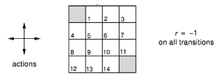
I’m currently learning Reinforcement Learning course by David Silver (here) and currently on studying lecture 3 and I find one particular example interesting. Taking it out of the context of RL and putting it simply, the example is to evaluate a random walk along a grid and find the expected number of steps required to reach some terminal nodes.
Solve by Simulation
Probably the most trivial way to calculate that is too just simulate it and find the average steps needed.
import random
import itertools


height, width = 4, 4
terminals = {(0,0), (3,3)}


grid = [[0 for i in range(height)] for j in range(width)]


for start_loc in itertools.product(range(height), range(width)):
	actions = [(0,1), (1,0), (0, -1), (-1, 0)]

	trial = 10000
	total_cost = 0
	for __ in range(trial):
		i, j = start_loc
		while (i, j) not in terminals:
			d_i, d_j = random.choice(actions)
			i += d_i
			j += d_j
			i = 3 if i > 3 else 0 if i < 0 else i
			j = 3 if j > 3 else 0 if j < 0 else j
			total_cost += 1
	grid[start_loc[0]][start_loc[1]] = total_cost/trial


def print_grid(grid):
	for row in grid:
		for column in row:
			print("%.3f\t" % column, end="")
		print()


print_grid(grid)
In the example above, I take the average of 10000 trials. (Note that if an action leads the walk to hit a wall, it just stays in place.) And the output I get is:
0.000	13.737	20.157	21.989
14.127	17.652	20.138	19.724
19.942	20.039	18.142	13.969
21.957	20.273	13.782	0.000
So if we start at the location (0, 1), we are about to hit a terminal nodes after roughly 13.733 steps, and roughly 21.989 step if we start at (0, 3).
Then what? What is interesting here is that we can get that number from other approach.
Solve by Iterative Policy Evaluation
The main step of iterative policy evaluation is to get the cost from averaging of the possible 4 previous parent actions. We first initialize all the cost (the expected step required) to be zero and build it up iteratively. It can be proven that it will converge to the actual expected value. Read http://www0.cs.ucl.ac.uk/staff/d.silver/web/Teaching_files/DP.pdf for more detailed explanation.
import itertools


def create_grid(height, width):
	return [[0 for i in range(height)] for j in range(width)]

def it_policy_eval(grid, terminals):
	new_grid = create_grid(height, width)
	for i, j in itertools.product(range(height), range(width)):
		if (i, j) in terminals:
			continue
		east_val = -1 + grid[min(i+1, 3)][j]
		west_val = -1 + grid[max(i-1, 0)][j]
		north_val = -1 + grid[i][min(j+1, 3)]
		south_val = -1 + grid[i][max(j-1, 0)]
		new_grid[i][j] = (east_val+west_val+north_val+south_val)/4
	return new_grid

def print_grid(grid):
	for row in grid:
		for column in row:
			print("%.3f\t" % column, end="")
		print()

height, width = 4, 4
grid = create_grid(height, width)

terminals = {(0,0), (3,3)}

k = 1000
for __ in range(k):
	grid = it_policy_eval(grid, terminals)
print_grid(grid)
As similarly indicated in the lecture notes, this is the value of of the grid evaluation for some values of k
k = 0
0.000	0.000	0.000	0.000
0.000	0.000	0.000	0.000
0.000	0.000	0.000	0.000
0.000	0.000	0.000	0.000


k = 1
0.000	-1.000	-1.000	-1.000
-1.000	-1.000	-1.000	-1.000
-1.000	-1.000	-1.000	-1.000
-1.000	-1.000	-1.000	0.000


k = 2
0.000	-2.438	-2.938	-3.000
-2.438	-2.875	-3.000	-2.938
-2.938	-3.000	-2.875	-2.438
-3.000	-2.938	-2.438	0.000


k = 3
0.000	-4.209	-5.510	-5.801
-4.209	-5.219	-5.590	-5.510
-5.510	-5.590	-5.219	-4.209
-5.801	-5.510	-4.209	0.000


k = 10
0.000	-8.337	-11.609	-12.610
-8.337	-10.608	-11.665	-11.609
-11.609	-11.665	-10.608	-8.337
-12.610	-11.609	-8.337	0.000


k = 1000
0.000	-14.000	-20.000	-22.000
-14.000	-18.000	-20.000	-20.000
-20.000	-20.000	-18.000	-14.000
-22.000	-20.000	-14.000	0.000
And we get the similar result as the result from the simulation.