How Regex is Matched

I have always wondered on how a regex like (a|b)*abb is matched with string like aabb (the regex pattern basically mean, match any number of a or b, followed with abb, like aaaaaabaabbaaaabb and abb). It may look obvious to us, but I start to wonder how does the regex matcher know whether the first a of aabb is matched to the (a|b)* and not to the a in abb before looking at the rest of the string? Another more confusing example is abbabb. How do they know to match the first abb in the string with the (a|b)*? I guessed that it will do some kind of trial and error and backtracking. That is possible, but how can be that logic be generated dynamically?

First step: state diagram

Turns out they don’t do a code path of logic and backtracking, but rather converting the regex expression to a graph (collection of states), and then try to match the string by going through the graph.

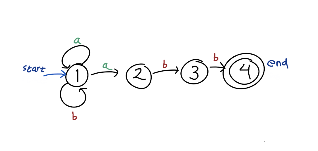
For example, the regex (a|b)*abb can be represented as: The graph above will contain all possible strings that match the regex pattern, represented as all possible paths from the start state to the end state.

But it still does not answer the question on why the first a in aabb is matched with the (a|b)*? Or in other words why the first a is used for transition from state 1 to 1 (through the self loop), instead of going to state 2? Turns out (or at least in this case), they don’t know. What they do is to try all path at the same time. Somewhat similar to breadth-first-search.

nodes = {
  1: {'a': [1, 2], 'b': [1], 'is_end': False},
  2: {'a': [], 'b': [3], 'is_end': False},
  3: {'a': [], 'b': [4], 'is_end': False},
  4: {'a': [], 'b': [], 'is_end': True}
}
def match(nodes, start_node, s):
    frontline = {start_node}
    for c in s:
        next_frontline = set()
        for node in frontline:
            next_frontline |= set(nodes[node][c])
        frontline = next_frontline
    for node in frontline:
        if nodes[node]['is_end']:
            return True
    return False

assert match(nodes, 1, 'abb')
assert match(nodes, 1, 'aabb')
assert match(nodes, 1, 'abbabb')
assert not match(nodes, 1, 'abbab')
assert not match(nodes, 1, 'aaaa')

In the algorithm shown above, frontline means all the possible state they can possibly after reading some part of the string. If there is no node at the frontline after reading the last character of string, then it will return false. It will also return false if no node in the last frontline has is_end equal to true.

Now it starts to make more sense. But we might notice that the algorithm may not perform really well if we have a lot of nodes at the frontline. There is the next step that we can do to improve it. We will modify the graph such that to check the string, we need exactly len(s) step.

Second Step: Deterministic State Diagram

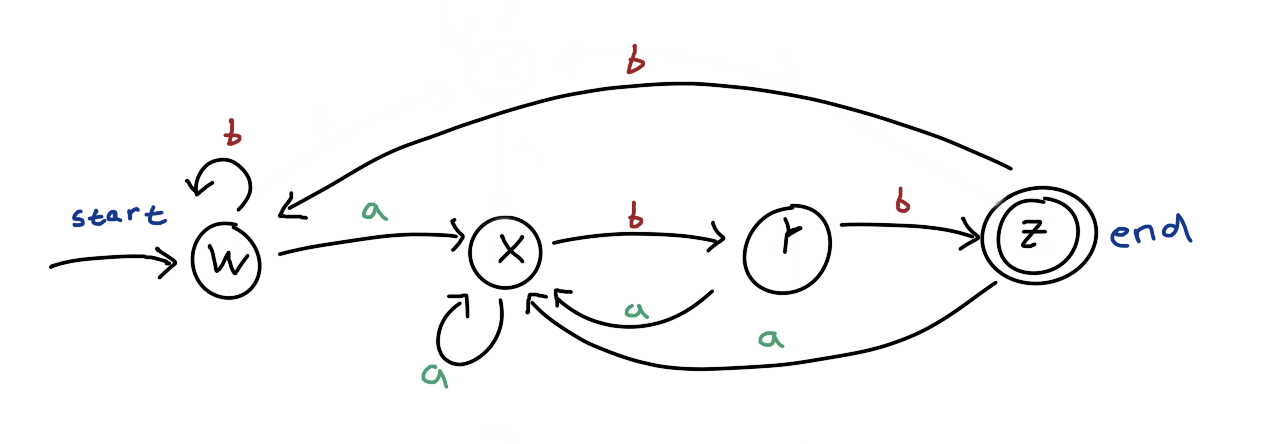
Before even studying about how can this graph came up, look at how clever it is. Try to trace the string abb, abbabb, and aaabbabb. And also see that ababbaab, and abab won’t be accepted (not ending at the “end” node).

The fundamental difference between this graph and the previous one is that it is deterministic, in a sense that for every state, the next state can be deterministically known given the next character c from string s (contrast it with the previous graph, state 1 may go to state 2 or keep at 1 if the next character is a). Because of that, we will always have the size of frontline to be at most one.

Regarding on how can we generate this graph, turns out that it is similar with the algorithm we used for the nondeterministic state diagram, but we just precompute it and “encode” it into states (and ignoring equivalent repetitive sub-paths). It may be a bit confusing at first, but things will be clearer when we see the example.

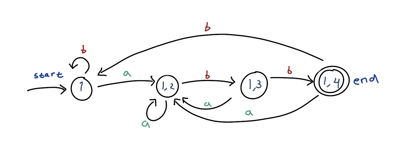
• We initially start with frontline of {1}. This corresponds to the state W in the deterministic graph.
• If we apply the trarsition a, we may end up in state 1 or 2. Hence the frontline {1, 2}. This corresponds to the state X. If we apply transition b instead, we get to {1} again , and this is no different than initial condition, hence the self-loop of transition b on W.
• In the state X (frontline {1, 2}), if we apply transition a, our frontline will be back to {1, 2} (the initial 2 get dropped and 1 yields to 1 and 2), because we can’t apply transition a on state 2. Thus the self-loop of transition a on X. But, if we apply transition b instead, our frontline will be {1, 3}. This is a new set of frontline. This corresponds with the state Y.
• In the state Y (frontline {1, 3}), applying a will get us to {1, 2} (1 yields to 1 and 2; 3 get dropped), hence going back to state X. Applying b will get us to {1, 4}. This is a new state again. This corresponds with the state Z.
• From Z ({1, 4}), applying a get us to {1, 2} or X, applying b get us to {1}, or W.

Basically, all the state in the deterministic graph represent subsets of states in the nondeterministic graph (a.k.a., the frontline). This is why I said that we are actually just precomputing and “encoding” the possible scenario of the execution of the nondeterministic graph matching. Though the runtime for matching the string with the graph is faster on the deterministic graph, we shifted the burden to the precomputation step of building the graph.

This is extracted from the textbook “Compilers: Principles, Techniques, and Tools” (Aho et al.). You can read more on section 3.6-3.7 for this topic. They provide a more rigorous explanation on this.